1. Introduction: Time Dynamics and Economics of the Injection Molding Cycle
Injection molding is one of the most widely used manufacturing processes in global polymer processing, and its economic performance and technical feasibility depend to a large extent on the control and optimization of "cycle time". Cycle time is the total time required to complete one full production sequence, from melting the polymer pellets, injecting them into the mold, cooling and solidifying, to finally ejecting the part. In the injection molding industry, a shorter cycle time means not only a linear increase in productivity, but is also directly linked to lower energy consumption and a maximized return on investment (ROI) in fixed assets. Compressing the cycle, however, is not an unbounded linear optimization problem; it is a multiphysics coupling problem strictly constrained by thermodynamics, rheology, mechanical mechanics, and the physical properties of the polymer material.
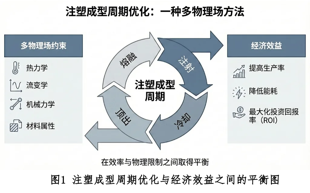
Traditional cycle time estimation often relies on empirical formulas or simple trial and error, which falls short when dealing with parts of complex geometry, sharply varying wall thickness, or high-performance engineering plastics. With the rapid advance of computational fluid dynamics (CFD), finite element analysis (FEM) and, more recently, artificial intelligence (AI), injection molding cycle modeling has evolved from a mere accumulation of experience into a precise science of mathematical and physical modeling.
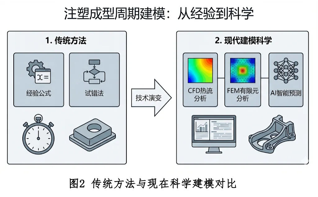
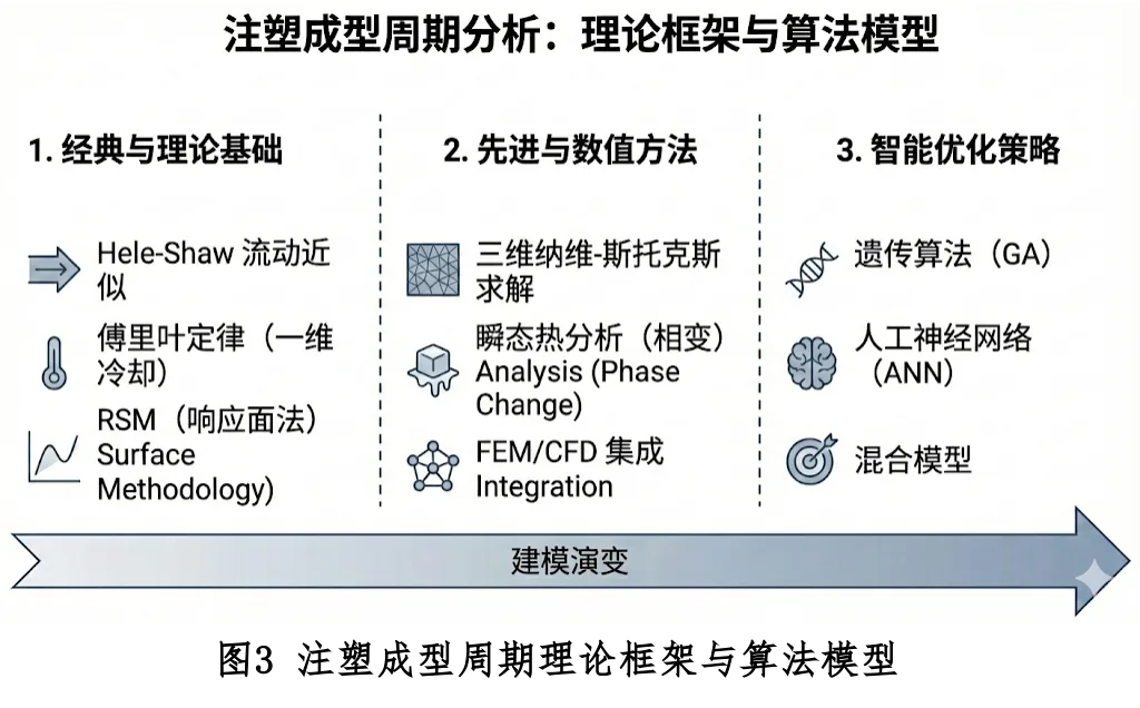
This article aims to provide a detailed analysis of the theoretical framework, governing equations and algorithmic models of each stage of the injection molding cycle. It explores in depth from the classical Hele-Shaw flow approximation to full three-dimensional Navier-Stokes solutions, from one-dimensional cooling models based on Fourier's law to transient thermal analysis including latent heat of phase change, and from traditional response surface methodology (RSM) to intelligent optimization strategies based on genetic algorithms (GA) and artificial neural networks (ANN).
 Strategies">
1.1 Composition and Interaction of the Molding Cycle
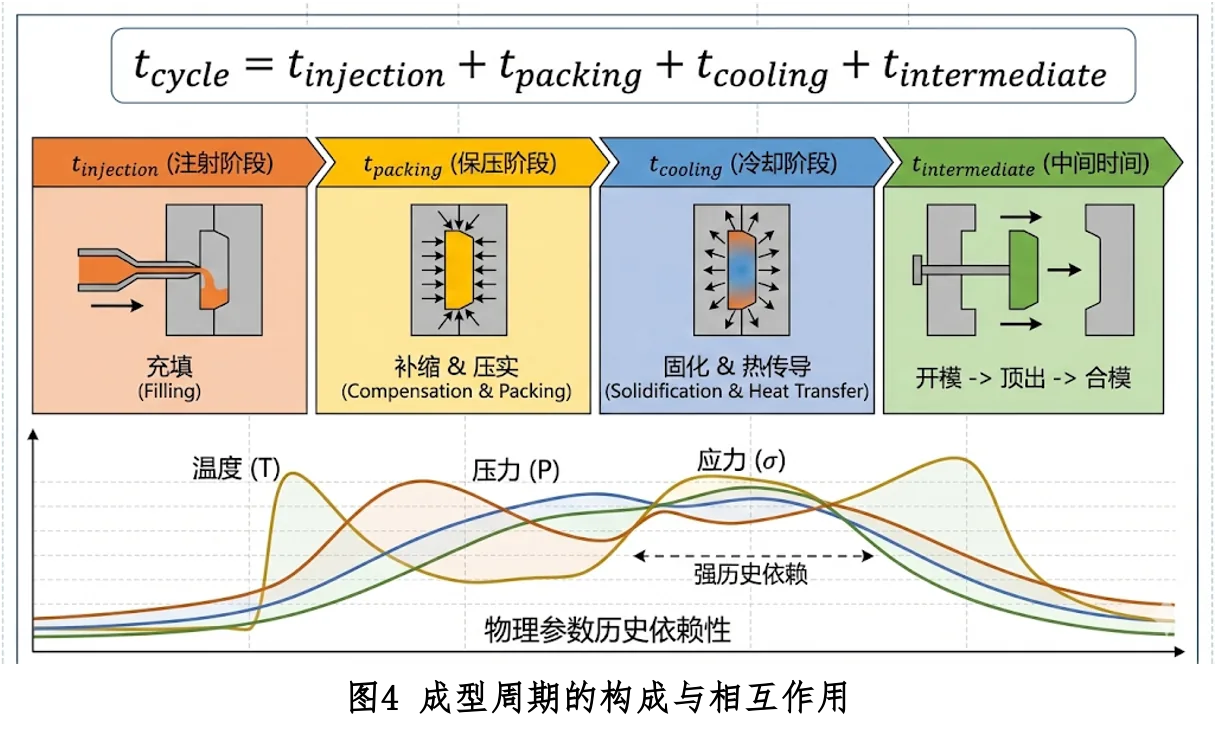
From the perspective of algorithmic modeling, the total cycle time $t_{cycle}$ is typically decomposed into four discrete yet physically tightly coupled stages. Although the stages are sequential along the time axis, their underlying physical parameters (e.g., temperature, pressure, stress) exhibit strong path dependence.
- $t_{injection}$ (Fill Time, $t_i$): the time required for the melt to fill the mold cavity. This stage is mainly controlled by hydrodynamic and rheological properties.
- $t_{packing}$ (Holding Time, $t_p$): the time during which melt is continuously injected to compensate for cooling shrinkage, until the gate freezes. This stage is governed by the polymer's pvT (pressure-specific volume-temperature) equation of state.
- $t_{cooling}$ (Cooling Time, $t_c$): the time for the polymer to release heat inside the mold until it reaches ejection rigidity. This is the longest part of the cycle, usually 60%–80% of the total, governed by the unsteady-state heat conduction equation.
- $t_{intermediate}$ (Intermediate/Auxiliary Time, $t_d$): includes mold opening, ejection, part removal, mold closing, and the machine's idle-cycle time. This stage is mainly limited by the injection machine's mechanical kinematics and the demolding friction mechanics of the part.
 ">
2. Fill-Stage Algorithm Model: Rheology and Fluid Dynamics
The filling stage is the starting point of the injection-molding cycle; its core task is to precisely pump the non-Newtonian fluid (polymer melt) into the complex mold cavity within an extremely short time. The prediction algorithm for fill time $t_{injection}$ must resolve the coupled evolution of the velocity, pressure, and temperature fields of the fluid during flow.
2.1 Governing Equations
In numerical simulation software (e.g., Moldflow, Moldex3D), the simulation of the filling process is based on the conservation laws of continuum mechanics.
2.1.1 Mass Conservation Equation
$$\frac{\partial \rho}{\partial t} + \nabla \cdot (\rho \mathbf{u}) = 0$$where $\rho$ is the fluid density and $\mathbf{u}$ is the velocity vector.
2.1.2 Momentum Conservation Equation (Navier-Stokes)
$$\rho \left( \frac{\partial \mathbf{u}}{\partial t} + \mathbf{u} \cdot \nabla \mathbf{u} \right) = -\nabla p + \nabla \cdot \boldsymbol{\tau} + \rho \mathbf{g}$$In classical injection-molding simulation algorithms, the Hele-Shaw approximation is typically adopted to simplify the above equations, assuming pressure is constant through the thickness and neglecting inertial terms.
2.1.3 Energy Conservation Equation
$$\rho c_p \left( \frac{\partial T}{\partial t} + \mathbf{u} \cdot \nabla T \right) = \nabla \cdot (k \nabla T) + \eta \dot{\gamma}^2$$Among them, the last term $\eta \dot{\gamma}^2$ represents viscous dissipation, which is crucial at high shear rates.
2.2 Rheological Constitutive Model
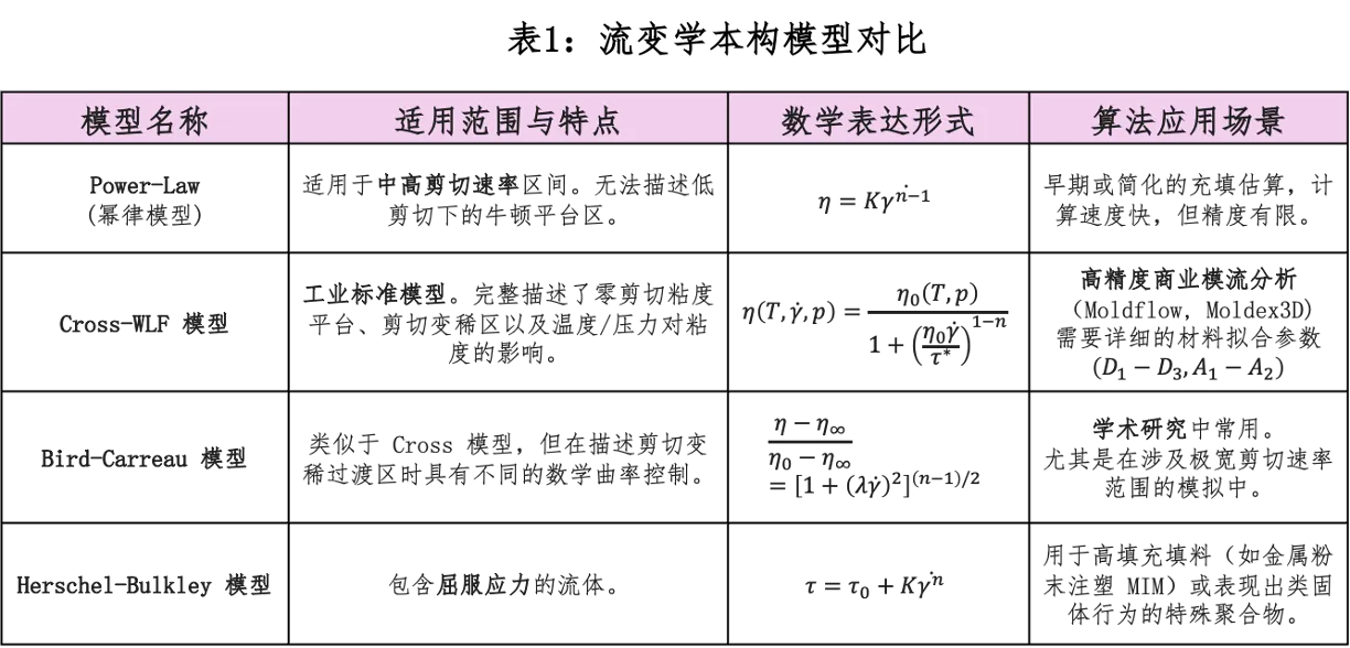
To close the system of equations, a constitutive equation must be introduced. The Cross-WLF model is the key link coupling the temperature and flow fields:
2.3 Fill Time Estimation Algorithm
Numerical simulation algorithms adopt the finite element (FEM) or finite volume (FVM) method, and precisely capture the gas–liquid interface position through flow front tracking algorithms such as VOF or Level Set.
3. Hold-Stage Algorithm Model: Compressibility and Shrinkage Compensation
Once the melt fills the cavity, the flow mechanism undergoes a fundamental shift. The algorithmic core of the holding-pressure stage is based on the polymer's pvT (pressure–specific volume–temperature) relationship.
3.1 pvT Equation of State
Dual-Domain Tait Equation is currently the most widely used model:
$$v(P, T) = v_0(T) \left( 1 - C \ln \left( 1 + \frac{P}{B(T)} \right) \right) + v_t(P, T)$$3.2 Gate Freeze-Off Time Prediction
The gate is judged frozen when the thermal criterion ($T_{gate} \leq T_{trans}$) and the rheological criterion (mass flow rate $|\dot{m}| < \epsilon$) are both satisfied.
3.3 Pressure Decay Model
$$P(t) = P_{initial} \cdot \exp\left(-\frac{t}{\tau_{relax}}\right)$$Accurately simulating this decay process is vital for predicting residual stress.
4. Cooling-Stage Algorithm Model: the Core Challenge of Heat Transfer
Cooling time $t_{cooling}$ accounts for 70%–80% of the molding cycle, and is the key to optimization.
4.1 One-dimensional unsteady heat conduction analytical model
Classic Flat-Plate Cooling Equation:
$$t_{cooling} = \frac{s^2}{\pi^2 \alpha_{eff}} \ln \left( \frac{4}{\pi} \cdot \frac{T_{melt} - T_{mold}}{T_{eject} - T_{mold}} \right)$$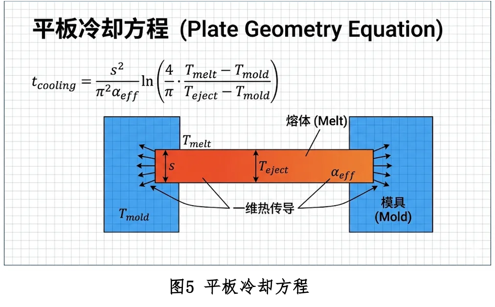
Key Insight: Cooling time is proportional to the square of wall thickness ($t_c \propto s^2$). Doubling the wall thickness quadruples the cooling time.
4.2 Advanced Thermodynamics Algorithm: Phase Change and Enthalpy Model
Accounting for the effect of crystallization latent heat $L$, use the effective specific heat $c_{p,eff}$:
$$c_{p,eff}(T) = c_p(T) + L \cdot \frac{d\chi}{dT}$$4.3 Conformal Cooling Channel Optimization
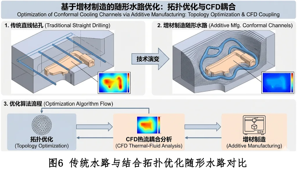
Through topology optimization and CFD thermal-flow coupling, conformal cooling systems can shorten cooling time by 30%–40%.
5. Ejection and Intermediate Stages: Mechanical and Kinematic Limits
The estimation model for ejection force $F_{eject}$ combines tribology and thermal-shrinkage principles:
$$F_{eject} = \mu \cdot P_{residual} \cdot A_{contact} + F_{vacuum}$$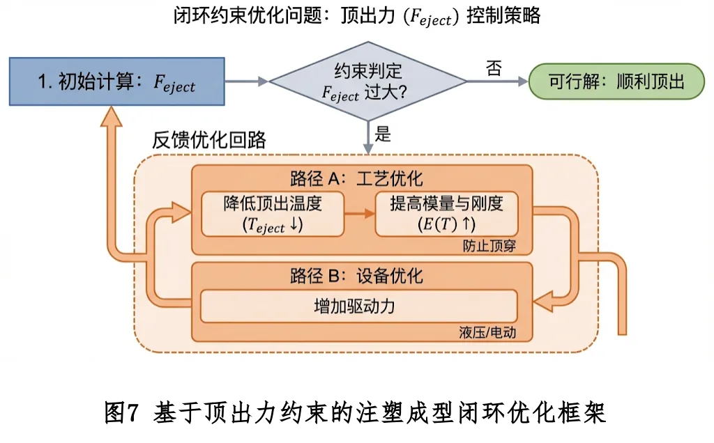
6. Numerical Simulation Architecture: Algorithm Implementation of FEM and FDM
To solve the above system of partial differential equations (PDEs) on a computer, they must be discretized. The core difference among injection-molding CAE software often lies in the choice of discretization algorithm.